Observability

During development, we follow a process and have many tools including functional tests (unit, integration, end-to-end), static analyzer, performance regression tests, and others before we ship to production. In spite of developers best effort, bugs do occur in production. Typical tools we have during development may not be applicable to a production setting. What we need is some visibility on our program’s internal state and how it behaves in production. For example, error logs can tell what is going on and include what user request looks like. An endpoint which is slow will need to be looked at, and it will be great if we can find out which one, and pinpoint exactly where the offending part of a codebase is. These data—or signals—are important to give us insight on what is going on with our applications. For the rest of this post, we will look at available tools to give us this visibility and help us solve this problem.

There are many tools, a crowded one, that provides visibility into not only how a program behaves, but can also report errors while a program is running in production. You may have heard of the term APM or application performance monitoring solutions like Splunk, Datadog, Amazon X-Ray, Sentry.io, ELK stack, and many others that provide complete (partial in some) end-to-end solution to peek under the hood and provide tools to developers to understand a program’s behaviour. These solutions work great. But sometimes we want the flexibility of switching to another vendor. It may be because we want features other vendor have, or it may be because of cost-saving. When we try to adopt one of these solutions, you might find it hard to migrate because of extensive changes needed to be done throughout a codebase, thus feeling locked into one ecosystem.

Thus came OpenTelemetry. It merges the efforts of OpenCensus and OpenTracing in the yesteryear into a single standard anyone can adopt so switching between vendors becomes easier. The term OpenTelemetry in this post encompasses the APIs, SDKs and tools to make up this ecosystem. Over the years, to my surprise, OpenTelemetry is being adopted by heavy hitters including the companies I mentioned above, as well as countless startups in the industry. This is great because when it becomes easy to switch, there is a greater incentive for these vendors to provide a better service and this only benefits developers and your company stakeholders. This is the promise of a vendor-neutral approach championed by cncf.io to ensure innovations are accessible for everyone.

Today, OpenTelemetry has advanced enough that I am comfortable at recommending them to any software programmers. OpenTelemetry has come a long way (and evolved over the years) so in this post, we will give a basic explanation of what OpenTelemetry is and an overview of how its observability signals work under the hood. Then we talk about how its collector tool works and how it helps in achieving vendor-neutrality.

Table of Contents

Observability Signals

Before we go deeper into implementation, we need to know what we are measuring or collecting. In OpenTelemetry world, these are called signals which includes metrics, tracing, and logs. These signals are the three pillars of OpenTelemetry.

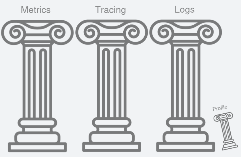
Figure 1: Greek pillars are what I imagine every time I hear the term three pillars of observability.

Logs are basically the printf or console.log() to display some internal messages or state of a program. This is what developers are most familiar with. It provides invaluable information at debugging.

Metrics represents aggregation of measurements of your system. For example, it can measure how big is the traffic to your site and its latency. These are useful indications to find out how your system performs. The measurement can be drilled down to each endpoint. So your system could have a 100% uptime by looking at your /ping endpoint, but it does not tell how each endpoint performs. Other than performance, you might be interested to know other measurements like the current total active logged-in users, or the number of user registrations in the past 24 hours.

Tracing may be the least understood tool as it is a relatively newer signal tool. Being able to pinpoint where exactly an error is happening is great—something that logs can do—but arriving to that subsystem can originate from multiple places (maybe from a different microservice). Moreover, an error can be unique to a request, so being able to trace the whole lifecycle of the request is an invaluable tool to find how the error came to be.

These are the central signals that we will dive into deeply. There is a fourth signal called profiling. Profiling has been with us for decades, and it is an invaluable tool during development that gives us means to see how much RAM and CPU cycles a particular function uses down to the line number. Profiling in this context refers to having these data live in a production setting (just like the other three signals), and across microservices! For now, profiling is in an infancy state, so we will focus on the other three signals.

Visualisation

Before diving deeper into the signals, it would be great to see if we can visualise what the end product could look like. The screenshot below is an example of an observability dashboard we can have. It gives us a quick glance on important information such as how our endpoints are doing, what logs are being printed, and some hardware statistics.

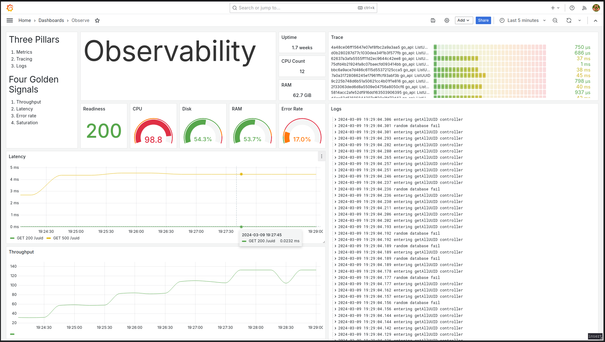Figure 2: Single pane of view to observability.

Now we will look into each of the pillars, so let us start with the most understood signal, namely logging.

Logging

When you have a program deployed on a single server, it is easy to view the logs by simply SSH-ing into the server and navigate into the logs directory. You may need some shell script skills in order to find and filter relevant lines pertaining to errors you are interested with. The problem comes when you are also deploying your program to multiple servers. Now you need to SSH to multiple servers in order to find the errors you are looking for. What’s worse is when you have multiple microservices, and you need to navigate to all of them just to find the error lines you want.

Figure 3: Have you ever missed the error lines you are interested with in spite of your shell script skills?

An easy solution is to simply send all of these logs into a central server. There are two ways of doing this; either the program pushes these logs to a central server, or you have another process that does the collecting and batching to send these logs. The second approach is what is recommended in the 12-factor app. We treat logs as a stream of data and log them to stdout, to be pushed to another place where we can tail and filter as needed. The responsibility of managing logs is handed over to another program. To push the logs, the industry standard is by using fluentd but there are other tools like its rewrite called Fluent Bit, otel-collector, logstash, and Promtail. Since this post is about OpenTelemetry, we will look at its tool called otel-collector.

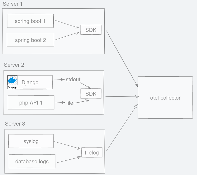Figure 4: No matter where logs are emitted, they can be channelled to otel-collector.

In the diagram above, Java spring boot app does not save the logs into a file. Instead, we have an option of an easy auto-instrumentation called OpenTelemetry javaagent SDK that automatically sends the logs to otel-collector.

A containerised application like the python Django application can have its logs tailed to be sent to otel-collector too. In reality, logs in containerised apps live in a place like /var/lib/docker/containers/<container_id>/*.log anyway. So, PHP logs like laravel which saves logs into files can be sent the same way to otel-collector.

Like many tools, otel-collector is flexible with where it can retrieve logs from. The log collection is not limited to API applications. Syslog and logs from the database can also be emitted to otel-collector.

This single otel-collector accepts a standardised API for logs. This means any vendor that can support OpenTelemetry can read your log output.

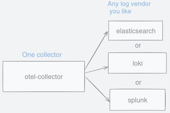Figure 5: Choose between any logging backend you like as long as they support otlp format.

Now that you have all logs in one place, you can search, filter by application or log level easily. OpenTelemetry’s solution automatically associates log entries with its origin which makes this an easy task.

Below screenshot shows a snippet of what a log aggregator like Loki can do. Here, I picked logs only for Laravel that have the word ‘ErrorException’ in it, formatted as json and only where the log level is more than 200. This query language is not standardised yet, but it already looks more readable than writing shell scripts with tail, awk, and grep.

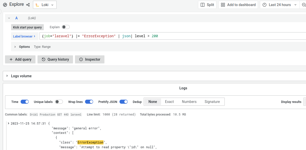Figure 6: Great user interface that allows searching using a readable query language.

Filtering the logs based on origin is not the only task OpenTelemetry supports. You will also be interested in finding out all logs from a particular request. This request can have a unique identifier, and we can associate this unique key to all logs in this particular request. The code below has a unique string (bcdf53g) right after log level being associated to a single request lifecycle for retrieving a list of authors from the database.

...
[2023-11-16 13:15:48] INFO bcdf53g listing authors
[2023-11-16 13:15:48] INFO e6c8af8 listing books
[2023-11-16 13:15:50] INFO bcdf53g retrieiving authors from database
[2023-11-16 13:15:51] ERROR bcdf53g database error ["[object] (Illuminate\\Database\\QueryException(code: 1045):
...

Now you can filter the logs for that particular request to get a better understanding of how the error came about.

{job="laravel"} |= bcdf53g

This returns only relevant log lines to you and eliminates the noise you do not care about.

...
[2023-11-16 13:15:48] INFO bcdf53g listing authors
[2023-11-16 13:15:50] INFO bcdf53g retrieiving authors from database
[2023-11-16 13:15:51] ERROR bcdf53g database error ["[object] (Illuminate\\Database\\QueryException(code: 1045):
...

More details about this unique key is covered in the tracing section. Also note that the logs do not always have to be in JSON format. The normal log line format shown above is still fine and most vendors provide the ability to filter and search this kind of format.

~~

Before moving on to the next signal, there is one thing of note which must be mentioned which is its SDK availability.

The OpenTelemetry SDK is fantastic if its SDK exists for your programming language. Recently, logs SDK has reached its stable 1.0 version and is generally available for most of the major programming languages.

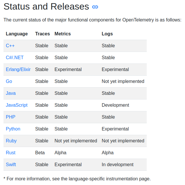Figure 7: https://opentelemetry.io/docs/instrumentation/#status-and-releases

But there are some glaring omission in this table. Considering many of observability programs are written in Go, its logs SDK for this language is missing. To make matter worse, there is no easy auto-instrumentation like Java is for Go. There are solutions to overcome this using eBPF like what Odigos and Grafana Beyla are doing which are worth keeping an eye on. Python is another major programming language which is at ‘Experimental’ stage. Nevertheless, there is always an alternative such as using a log forwarder like fluentd or Promtail. You might want to ensure the tools you use is otlp-compatible so that you do not have to re-instrument your code base in the future.

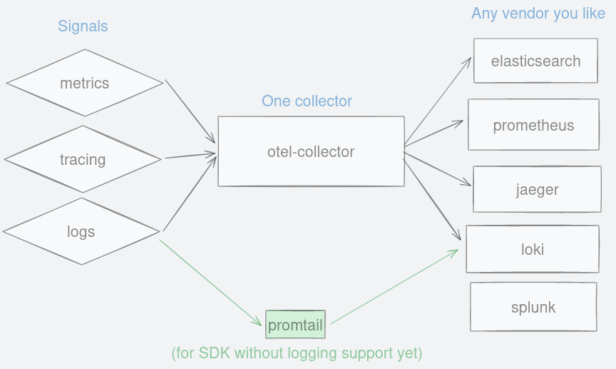Figure 8: Alternative pathway for pushing logs into your backend using promtail.

Metrics

According to the 4 Golden Signals for monitoring systems, we measure traffic, latency, errors and saturation. For metrics, we care about RED method which are Rate, Errors, and Duration.

Just like logging where logs are channelled to a central place, metrics data are also aggregated through otel-collector and then exposed as an endpoint. By default, metrics data are accessed from otel-collector through http://localhost:8889/metrics. This is the endpoint that a vendor like Prometheus uses to scrape metrics data at a regular interval. Let us have a look at what these metrics data look like.

Let us make a single request to a freshly instrumented application. For example:

curl -v http://localhost:3080/uuid

Then visit the endpoint exposed by otel-collector at http://localhost:8889/metrics to view metrics data. The data being returned is in plaintext (text/plain) with a certain format.

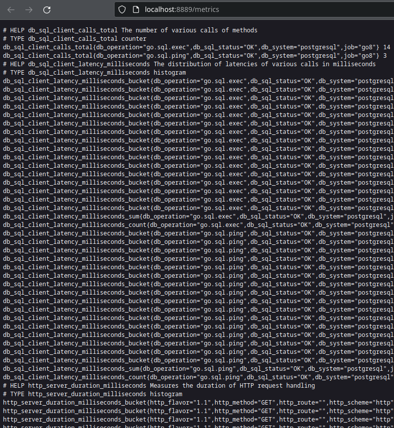Figure 9: Raw metrics data collected by otel-collector.

For now, we are interested in finding out the request counter. So do a search with Ctrl+F for the metric name called http_server_duration_milliseconds_count.

http_server_duration_milliseconds_count{http_method="GET",http_route="/uuid",http_scheme="http",http_status_code="200",job="java_api",net_host_name="java-api",net_host_port="8080",net_protocol_name="http",net_protocol_version="1.1"} 1

Inside this metric, it contains several labels in a key="value" format separated by commas. It tells us that this metric records the /uuid endpoint for a GET request. It also tells us this is for a job called java_api. This job label is important because we could have the same metric name in other APIs, so we need a way to differentiate this data. At the end of the line, we have got a value of 1. Try to re-run the api call once more, and watch how this value changes.

curl -v http://localhost:3080/uuid

Refresh and look for the same metric for /uuid endpoint. You will see that the value has changed.

http_server_duration_milliseconds_count{...cut for brevity...} 2

Notice that at the end of the line, the value has changed from 1 to 2.

So how does this measure the rate? A rate is simply a measurement of change that occurs over time. There was a lag that happened between the first time you called /uuid end point and the second. Prometheus uses this duration and collects the value in order to find out the rate. Easy math!

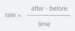Figure 10: Formula to finding out the rate is simply the delta over time.

~~

What about latency? The amount of time it took to complete a request is stored into buckets. To understand this, let us take it step-by-step. For this api, Prometheus stores the latency in histograms. Let us construct a hypothetical one:

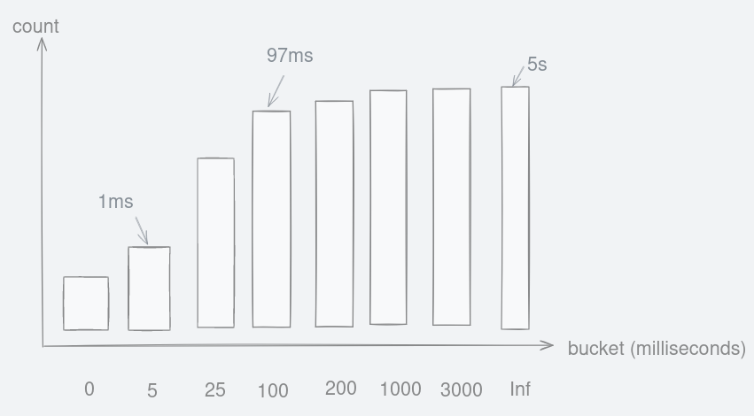Figure 11: Hypothetical cumulative histogram that stores request duration into buckets.

If a request took 97 milliseconds, it will be placed inside the fourth bar from the left because it was between 25 and 100. So the count increased for this bar labelled as ‘100’.

Anything lower than five milliseconds will be placed in the ‘5’ bucket. On the other extreme, any requests that take longer than three seconds get placed in the infinity(‘inf’) bucket.

Take a look back at the http://localhost:8889/metrics endpoint. I deleted many labels keeping only the relevant ones, so it is easier to see:

http_server_duration_milliseconds_bucket{http_route="/uuid",le="0"} 0
http_server_duration_milliseconds_bucket{http_route="/uuid",le="5"} 0
http_server_duration_milliseconds_bucket{http_route="/uuid",le="10"} 1
http_server_duration_milliseconds_bucket{http_route="/uuid",le="25"} 1
http_server_duration_milliseconds_bucket{http_route="/uuid",le="50"} 1
http_server_duration_milliseconds_bucket{http_route="/uuid",le="75"} 1
http_server_duration_milliseconds_bucket{http_route="/uuid",le="100"} 1
http_server_duration_milliseconds_bucket{http_route="/uuid",le="250"} 2
http_server_duration_milliseconds_bucket{http_route="/uuid",le="500"} 2

From the raw data above we can see that there is one request that took between 5 and 10 milliseconds. And another between 100ms and 250ms. What is strange is that there are values for bars such as ‘250’ and ‘500’. Value for bar ‘10’ is one because when a request latency is between 5ms and 10ms. The bar for ‘250’ is also one because it is also true that that request is less than or equal (le) to 10(!). The same reasoning applies to bar ‘500’. This type of histogram which is used by Prometheus is called cumulative and the ’le’ labels were predefined or fixed-boundaries.

This is such a simple example but should give you enough intuition on how they store data into histogram buckets.

~~

Now that we understand how Prometheus calculates rates and latency, let us visualise these. But first we need to use some query languages to translate what we want into something Prometheus understands. This query language is called PromQL.

Going into Prometheus’ web UI at http://localhost:9090, type in the following PromQL query. We re-use the same metric which is http_server_duration_milliseconds_count. Then we wrap the whole metric with a special function called rate(), and we want a moving or sliding calculation over one minute.

rate( http_server_duration_milliseconds_count{ job="java_api" } [1m] )

Using PromQL like above, we get fancy stuff like line charts for latency and throughput. You can view the line chart by clicking on the ‘Graph’ tab. But visualising from the provided Grafana dashboard looks nicer.

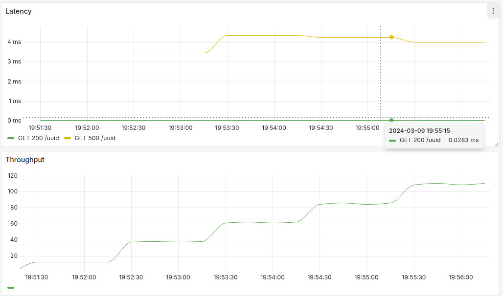Figure 12: Line charts showing latency and throughput for /uuid endpoint.

On the top half of the screenshot above, it shows latency for /uuid endpoint. Green line shows a 200 HTTP status response while the yellow line shows a 500 HTTP status response. Success response stays below 1 millisecond while error response is around 4 milliseconds. The lines can be hovered to see more details.

On the bottom half, it shows throughput or the rate/second. The graph shows an increasing throughput over time which reflects our synthetic load generator slowly increasing the number of users.

Prometheus support in your architecture

Web applications are not the only thing it can measure. Your managed database may already come with Prometheus support. Typically, such metrics are exposed by your service with /metrics endpoint so check out the documentation of your software of choice and you might be able to play with Prometheus right now.

Caveat

Metrics are great but the way it collects them produces a downside. If you look closely in both rate and latency calculations, there is always a mismatch between when something has happened and when Prometheus recorded these events. This is just the nature of Prometheus because it aggregates the states at a certain period in time. It does not record every single event like InfluxDB does. On the flip side, storing metrics data becomes cheap.

More

We have only talked about one type of measurement which is histogram. But it can also measure other types.

• Counters can be used to record increasing amounts of data points. For example, counting site visits.
• Gauge can be used for data points that can continuously increase and decrease. For example, CPU or RAM usage.

Tracing

As mentioned at the start of this post, knowing where an error occurred is great but what is better is knowing the path it took to arrive at the particular line of code. If you think this sounds like a stack trace, it is close! A stack trace shows functions that were called to arrive at a specific offending code. What is so special about tracing in observability? You are not limited to a single program, but you have the ability to follow a request flow across all of your microservices. This is called distributed tracing.

But first, let us start with a basic tracing and visualise using a time axis below through Grafana UI.

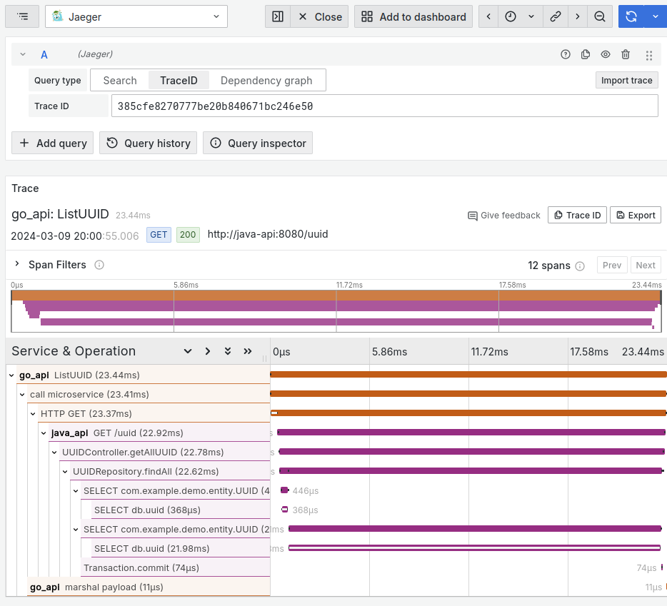Figure 13: Name and duration of twelve spans for this single trace of this request.

There are a lot going on but let us focus on what’s important. Every single trace (a unique request), has a random identifier represented by its hex value called trace ID. In the diagram above, it is 385cfe8270777be20b840671bc246e50. This trace ID is randomly generated for each request by the OpenTelemetry library.

Under the ‘Trace’ section, we see a chart with twelve horizontal dual-coloured bar graphs. These bars are called spans, and they belong to the single trace above. A span can mean anything, but typically we create one span for a one unit of work. The span variable you see in the code block below was created for the ListUUID() function. Using a manual instrumentation approach, we have to manually write a code to create a span, let the program do the work, then call span.End() before the function exits to actually emit the span to the otel-collector.

// api.go

func (s *Server) ListUUID(w http.ResponseWriter, r *http.Request) {
	tracer := otel.Tracer("")
	ctx, span := tracer.Start(r.Context(), "ListUUID")
	defer span.End()
	
	// do the work	

A span can belong to another span. In the trace graph above, we created a child span called “call microservice” for “ListUUID”. And because we performed an HTTP call to the java api, a span is automatically created for us.

Once the request went into the java API, all spans were created automatically thanks to auto-instrumentation. We can see the functions that were called, as well as any SQL queries that were made.

Each span not only shows parent-child relationship, but also the duration. This is invaluable to knowing possible bottlenecks across all of your microservices. We can see the majority of time was spent on the span called ‘SELECT db.uuid’ which took 21.98 milliseconds out of 23.44 milliseconds total of this request. That span can be clicked to display more details in the expanded view.

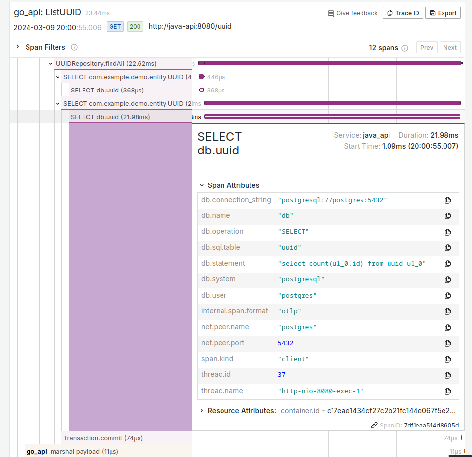Figure 14: Each span can be clicked to reveal more information.

Here we see several attributes including the database query. At the bottom, we see this span’s identifier which is 7df1eaa514d8605d.

Thanks to visualisation of the spans, it is easy to spot which part of the code took the most time. Drilling down which part of the code is slow is great, but 23.4 millisecond response time for a user-facing request is not something to be concerned with. The user interface allows us to filter slow requests by using the search button. For example, we can put a minimum duration of 500 milliseconds into the search filter form.

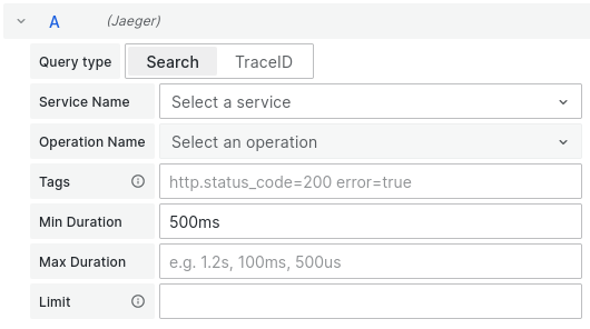Figure 15: Spans can be filtered to your criteria.

This way, we can catch slow requests, and have the ability to see the breakdown of which part of the code took most of the time.

Automatic Instrumentation

So tracing is great. But to manually insert instrumentation code into each function can be tedious. We did manual instrumentation for the Go api which was fine because we did not have to do many. Fortunately, code can be instrumented automatically without touching your codebase in several languages.

In languages where it depends on an interpreter (like Python) or Java VM (like this java demo API), bytecode can be injected to capture these OpenTelemetry signals. For example in Java, simply supply a path to a Java Agent, and set any config from either the startup command line or environment variable to your existing codebase.

java -javaagent:path/to/opentelemetry-javaagent.jar -Dotel.service.name=your-service-name -jar myapp.jar

Programs that compile into binaries are harder. In this case, eBPF-based solution like Odigos and Beyla can be used.

Sampling Traces

Unlike Prometheus where it aggregates records, we could store every single trace into the storage. Storing all of them will likely blow your storage limits. You will find that many individual traces are nearly identical. For that reason, you might want to sample the traces, say, only store ten percent of the traces. However, be careful of this technique because the trace you are interested in might lose its parent context because it selects traces at random. For that reason, trace SDK provides several sampling rules (https://opentelemetry.io/docs/concepts/sdk-configuration/general-sdk-configuration/#otel_traces_sampler). Sampling this way still means it is possible to miss an error happening in the system.

Distributed Tracing

As demonstrated with the demo repository, I have shown distributed tracing across two microservices. To achieve this, each service must be instrumented with OpenTelemetry SDK. Then when making a call to another microservice, span context is attached to outgoing requests for the receiving end to extract and consume.

~~

I hope this demystifies what tracing is. There are more things to learn so a great place to look is its documentation as https://opentelemetry.io/docs/concepts/signals/traces/.

Single Collector

Implementing OpenTelemetry into a program is termed as instrumenting. It can be done either manually, or automatically. Manually means writing lines of code into the functions to retrieve and emit both traces and spans.

Automatic instrumentation means either not touching the code at all or very minimal depending on the language. Approaches include using eBPF, or through runtime like Java’s approach to using JavaAgent, or an extension for php.

In either case, vendor-neutrality means your application only needs to be instrumented once using an open standard SDK. You may change vendors but your codebase stays untouched. All these signals are funnelled into a single collector before they are dispersed to OpenTelemetry-compatible destinations. Thanks to this SDK, you have fewer things to worry about when moving to another vendor.

As this is an open standard, otel-collector is not the only tool available out there. Alternatives like grafana agent exists too.

Now that we have OpenTelemetry signals in otlp format, any vendor that understands this protocol can be used. You have a growing choice of vendors at your disposal, open source or commercial, including Splunk, Grafana, SigNoz, Elasticsearch, Honeycomb, Lightstep, DataDog and many others.

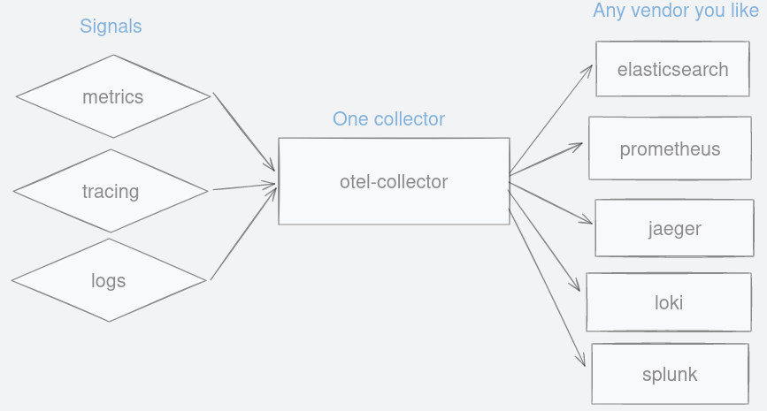Figure 16: A single collector to forward observability signals to any vendor you like.

Having a single component does not look good architecture-wise because it can become a bottleneck. In this context, it only means standardising the format so that anyone can write and read from it.

One deployment strategy is you can have multiple instances of otel-collector to scale it horizontally by putting a load balancer in front of it. Another popular approach is to have one otel-collector sit next to each of your programs like a sidecar. You can even put a queue in between otel-collector and vendors to handle load spikes.

Otel-Collector Components

As everything goes through otel-collector, let us talk one layer deeper about its components namely receivers, processors, exporters, and pipelines.

Receivers are how an otel-collector receives any observability signals. In the config file, we define a receiver called otlp using both gRPC and http as its protocol. By default, otel-collector listens at port 4317 and 4318 for HTTP and gRPC respectively.

# otel-collector-config.yaml

receivers:
  otlp:
    protocols:
      grpc:
      http:

Processors are how data is transformed inside the collector before being sent out. You can optionally batch them and have some memory limit. Full list of processors are in https://github.com/open-telemetry/opentelemetry-collector/tree/main/processor and contrib repo. Rate limiter is not in one of the processors so at a higher scale. A third party queue that sits in between otel-collector and vendors might be needed to alleviate possible bottlenecks.

# otel-collector-config.yaml

processors:
  batch:
  memory_limiter:

Exporters are how we define where to send these signals to. Here we have three. Metrics are being sent to Prometheus which is fast becoming the de-facto industry standard for metrics. Tracing, which is labelled as otlp will be sent to Jaeger while logs and sent to a URL. As you can see, switching your backend from one to another is as easy as swapping a new exporter(vendor) into this file.

# otel-collector-config.yaml

exporters:
  prometheus:
    endpoint: otel-collector:8889

  debug:
    verbosity: detailed
    endpoint: http://loki:3100/loki/api/v1/push

  otlp:
    endpoint: jaeger-all-in-one:4317

If you want to emit to multiple vendors, that can be done too. Simply add a suffix preceded with a slash (like /2) to it. Below, we can choose to send logs to both loki and dataprepper using ‘otlp/logs’.

# otel-collector-config.yaml

exporters:
  prometheus:
    endpoint: otel-collector:8889

  debug:
    verbosity: detailed
    endpoint: http://loki:3100/loki/api/v1/push
       
  otlp/logs:
     endpoint: dataprepper:21892
     tls:
        insecure: true

  otlp:
    endpoint: jaeger-all-in-one:4317

Metrics data are exposed as an endpoint at otel-collector:8889/metrics. For vendors who have OpenTelemetry protocol (otlp) support, these metrics can be pushed straight from otel-collector. For example, metrics can be pushed straight to Prometheus using http://prometheus:9090/otlp/v1/metrics endpoint.

Pipeline is the binding component that defines how data flows from one to another. Each of trace, metrics, and logs describes where to pull data, any processing needs to be done, and where to put the data to.

Lastly, Extensions can be applied to collect otel-collector’s performance. Examples are listed in the repository including profiling, zPages, and others.

# otel-collector-config.yaml

service:

  extensions: [pprof, zpages, health_check]
  
  pipelines:
    traces:
      receivers: [otlp]
      processors: [batch, memory_limiter]
      exporters: [debug, otlp]
    metrics:
      receivers: [otlp]
      processors: [batch, memory_limiter]
      exporters: [debug, prometheus]
    logs:
      receivers: [otlp]
      exporters: [debug, loki]

Having a single component that funnels data into otel-collector is great because when you want to switch to another log vendor, you can just simply add the vendor name into the logs’ exporters array in this configuration file.

Vendor Neutrality

A great deal of effort has been made to ensure vendor-neutrality in terms of instrumentation and OpenTelemetry protocol support. A standard SDK means you can instrument your code once, be that automatic or manual. Vendors supporting otlp means you can pick another vendor of your choosing easily by adding or swapping in your yaml file. The other two important parts to achieving vendor-neutrality are dashboards and alerting. Note that these components are not part of OpenTelemetry, but it is important to discuss this part of the ecosystem as a whole.

Both Prometheus and Jaeger have their own UI at http://localhost:9090 and http://localhost:16686 respectively. However, it is easier to have all information in one screen rather than shuffling between different tabs. Grafana makes this easy, and it comes with a lot of bells and whistles too. It gives the information I want, and they look great. However, are those visualisations portable if I want to switch to another vendor?

Take this case with Prometheus. Data visualisation is done using its query language called PromQL. While it may be the dominant metrics solution, competing vendor might have a different idea on the DSL to create visualisations. The same goes with querying logs—there isn’t a standard yet. For this, a working group to create a standardised, unified language has been started.

Second concern is alerting. It is crucial because when an issue arises in your application—latency for a specific endpoint passes certain threshold—it needs to be acted upon. You can measure response times using metrics like Mean Time to Acknowledge (MTTA), Mean Time to Resolve(MTTR) and others can be crucial for your service level agreement (SLA). Performing within SLA margins makes happy customers and pockets.

Alerting rules you have made in one vendor might not be portable to another since a standard does not exist.

Conclusion

In this post, we have learned about three important OpenTelemetry signals which are logs, metrics, and tracing. OpenTelemetry SDKs made it easy to instrument your application in your favourite language. Then we talked about otel-collector which receives, transforms and emits these signals through a standard API. Vendors that support OpenTelemetry protocol give us the freedom to pick and choose however we like without concern of re-instrumenting our codebase.

The approach OpenTelemetry is taking achieves vendor-neutrality which benefits everyone. For developers, it takes out the headache of re-coding. For business owners, it can be a cost-saving measure. For vendors, rising popularity means more potential customers come into this observability space.

For many years, OpenTelemetry project has been the second most active CNCF project right behind kubernetes amongst hundreds. It is maturing fast and it is great to see the industry working together for the common good.

Figure 17: OpenTelemetry belongs to CNCF.

Further Reads

Spec Overview https://github.com/open-telemetry/opentelemetry-specification/blob/main/specification/overview.md

CNCF projects https://landscape.cncf.io/